|
Rank Randomization: Two Conditions (Mann-Whitney U, Wilcoxon Rank Sum)
Author(s)
David M. Lane
Prerequisites
Permutations and Combinations, Randomization Tests for Two Conditions
Learning Objectives
- State the difference between a randomization test and a rank randomization test
- Describe why rank randomization tests are more common
- Be able to compute a Mann-Whitney U test
The major problem with randomization tests is that they are very difficult to compute. Rank randomization tests are performed by first converting the scores to ranks and then computing a randomization test. The primary advantage of rank randomization tests is that there are tables that can be used to determine significance. The disadvantage is that some information is lost when the numbers are converted to ranks. Therefore, rank randomization tests are generally less powerful than randomization tests based on the original numbers.
There are several names for rank randomization tests for differences in central tendency. The two most common are the
Mann-Whitney U test and the Wilcoxon Rank Sum test.
Consider the data shown in Table 1 that were used as an example in the section on randomization tests.
Table 1. Fictitious data.
| Experimental |
Control |
7
8
11
30 |
0
2
5
9 |
A rank randomization test on these data begins by converting the numbers to ranks.
Table 2. Fictitious data converted to ranks. Rank sum = 24.
| Experimental |
Control |
4
5
7
8 |
1
2
3
6 |
The probability value is determined by computing the proportion of the possible arrangements of these ranks that result in a difference between ranks as large or larger than those in the actual data (Table 2). Since the sum of the ranks (the numbers 1-8) is a constant (36 in this case), we can use the computational shortcut of finding the proportion of arrangements for which the sum of the ranks in the Experimental Group is as high or higher than the sum here (4 + 5 + 7 + 8 = 24).
First, consider how many ways the 8 values could be divided into two sets of 4. We can apply the formula from the section on Permutations and Combinations for the number of combinations of n items taken r at a time (n = the total number of observations; r = the number of observations in the first group) and find that there are 70 ways. 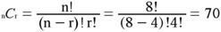
Of these 70 ways of dividing the data, how many result in a sum of ranks of 24 or more? Tables 3-5 show three rearrangements that would lead to a rank sum of 24 or larger.
Table 3. Rearrangement of data converted to ranks. Rank sum = 26.
| Experimental |
Control |
6
5
7
8 |
1
2
3
4 |
Table 4. Rearrangement of data converted to ranks. Rank sum = 25.
| Experimental |
Control |
4
6
7
8 |
1
2
3
5 |
Table 5. Rearrangement of data converted to ranks. Rank sum = 24.
| Experimental |
Control |
3
6
7
8 |
1
2
4
5 |
Therefore, the actual data represent 1 arrangement with a rank sum of 24 or more and the 3 arrangements represent three others. Therefore, there are 4 arrangements with a rank sum of 24 or more. This makes the probability equal to 4/70 = 0.057. Since only one direction of difference is considered (Experimental larger than Control), this is a one-tailed probability. The two-tailed probability is (2)(0.057) = 0.114 since there are 8/70 ways to arrange the data so that the sum of the ranks is either (a) as large or larger or (b) as small or smaller than the sum found for the actual data.
The beginning of this section stated that rank randomization tests were easier to compute than randomization tests because tables are available for rank randomization tests. Table 6 can be used to obtain the critical values for equal sample sizes of 4-10.
Table for unequal sample sizes (in a new window).
For the present data, both n1 and n2 = 4 so, as can be determined from the table, the rank sum for the Experimental Group must be at least 25 for the difference to be significant at the 0.05 level (one-tailed). Since the sum of ranks equals 24, the probability value is somewhat above 0.05. In fact, by counting the arrangements with the sum of ranks greater than or equal to 24, we found that the probability value is 0.057. Naturally a table can only give the critical value rather than the p value itself. However, with a larger sample size such as 10 subjects per group, it becomes very time-consuming to count all arrangements equaling or exceeding the rank sum of the data. Therefore, for practical reasons, the critical value sometimes suffices.
Table 6. Critical values.
One-Tailed Test
Rank Sum for Higher Group
|
| n1 |
n2 |
0.20 |
0.10 |
0.05 |
0.025 |
0.01 |
0.005 |
| 4 |
4 |
22 |
23 |
25
|
26
|
.
|
.
|
| 5 |
5 |
33 |
35 |
36 |
38 |
39 |
40 |
| 6 |
6 |
45 |
48 |
50 |
52 |
54 |
55 |
| 7 |
7 |
60 |
64 |
66 |
69 |
71 |
73 |
| 8 |
8 |
77 |
81 |
85 |
87 |
91 |
93 |
| 9 |
9 |
96 |
101 |
105 |
109 |
112 |
115 |
| 10 |
10 |
117 |
123 |
128 |
132 |
136 |
139 |
For larger sample sizes than covered in the tables, you can use the following expression that is approximately normally distributed for moderate to large sample sizes.
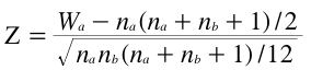
where:
Wa is the sum of the ranks for the first group
na is the sample size for the first group
nb is the sample size for the second group
Z is the test statistic
The probability value can be determined from Z using the normal distribution calculator.
The data from the Stereograms Case Study can be analyzed using this test. For these data, the sum of the ranks for Group 1 (Wa) is 1911, the sample size for Group 1 (na) is 43, and the sample size for Group 2 (nb) is 35. Plugging these values into the formula results in a Z of 2.13, which has a two-tailed p of 0.033.
Please answer the questions:
|