|
Introduction to Multiple Regression
Author(s)
David M. Lane
Prerequisites
Simple Linear Regression, Partitioning Sums of Squares, Standard Error of the Estimate, Inferential Statistics for b and r
Learning Objectives
- State the regression equation
- Define "regression coefficient"
- Define "beta weight"
- Explain what R is and how it is related to r
- Explain why a regression weight is called a "partial slope"
- Explain why the sum of squares explained in a multiple regression model is usually less than the sum of the sums of squares in simple regression
- Define R2 in terms of proportion explained
- Test R2 for significance
- Test the difference between a complete and reduced model for significance
- State the assumptions of multiple regression and specify which aspects of the analysis require assumptions
In simple linear regression, a criterion variable is predicted from one predictor variable. In multiple regression, the criterion is predicted by two or more variables. For example, in the SAT case study, you might want to predict a student's university grade point average on the basis of their High-School GPA (HSGPA) and their total SAT score (verbal + math). The basic idea is to find a linear combination of HSGPA and SAT that best predicts University GPA (UGPA). That is, the problem is to find the values of b1 and b2 in the equation shown below that give the best predictions of UGPA. As in the case of simple linear regression, we define the best predictions as the predictions that minimize the squared errors of prediction.
UGPA' = b1HSGPA + b2SAT + A
where UGPA' is the predicted value of University GPA and A is a constant. For these data, the best prediction equation is shown below:
UGPA' = 0.541 x HSGPA + 0.008 x SAT + 0.540
In other words, to compute the prediction of a student's University GPA, you add up (a) their High-School GPA multiplied by 0.541, (b) their SAT multiplied by 0.008, and (c) 0.540. Table 1 shows the data and predictions for the first five students in the dataset.
Table 1. Data and Predictions.
| HSGPA |
SAT |
UGPA' |
| 3.45 |
1232 |
3.38 |
| 2.78 |
1070 |
2.89 |
| 2.52 |
1086 |
2.76 |
| 3.67 |
1287 |
3.55 |
| 3.24 |
1130 |
3.19 |
The values of b (b1 and b2) are sometimes called "regression coefficients" and sometimes called "regression weights." These two terms are synonymous.
The multiple correlation (R) is equal to the correlation between the predicted scores and the actual scores. In this example, it is the correlation between UGPA' and UGPA, which turns out to be 0.79. That is, R = 0.79. Note that R will never be negative since if there are negative correlations between the predictor variables and the criterion, the regression weights will be negative so that the correlation between the predicted and actual scores will be positive.
Interpretation of Regression Coefficients
A regression coefficient in multiple regression is the slope of the linear relationship between the criterion variable and the part of a predictor variable that is independent of all other predictor variables. In this example, the regression coefficient for HSGPA can be computed by first predicting HSGPA from SAT and saving the errors of prediction (the differences between HSGPA and HSGPA'). These errors of prediction are called "residuals" since they are what is left over in HSGPA after the predictions from SAT are subtracted, and represent the part of HSGPA that is independent of SAT. These residuals are referred to as HSGPA.SAT, which means they are the residuals in HSGPA after having been predicted by SAT. The correlation between HSGPA.SAT and SAT is necessarily 0.
The final step in computing the regression coefficient is to find the slope of the relationship between these residuals and UGPA. This slope is the regression coefficient for HSGPA. The following equation is used to predict HSGPA from SAT:
HSGPA' = -1.314 + 0.0036 x SAT
The residuals are then computed as:
HSGPA - HSGPA'
The linear regression equation for the prediction of UGPA by the residuals is
UGPA' = 0.541 x HSGPA.SAT + 3.173
Notice that the slope (0.541) is the same value given previously for b1 in the multiple regression equation.
This means that the regression coefficient for HSGPA is the slope of the relationship between the criterion variable and the part of HSGPA that is independent of (uncorrelated with) the other predictor variables. It represents the change in the criterion variable associated with a change of one in the predictor variable when all other predictor variables are held constant. Since the regression coefficient for HSGPA is 0.54, this means that, holding SAT constant, a change of one in HSGPA is associated with a change of 0.54 in UGPA'. If two students had the same SAT and differed in HSGPA by 2, then you would predict they would differ in UGPA by (2)(0.54) = 1.08. Similarly, if they differed by 0.5, then you would predict they would differ by (0.50)(0.54) = 0.27.
The slope of the relationship between the part of a predictor variable independent of other predictor variables and the criterion is its partial slope. Thus the regression coefficient of 0.541 for HSGPA and the regression coefficient of 0.008 for SAT are partial slopes. Each partial slope represents the relationship between the predictor variable and the criterion holding constant all of the other predictor variables.
It is difficult to compare the coefficients for different variables directly because they are measured on different scales. A difference of 1 in HSGPA is a fairly large difference, whereas a difference of 1 on the SAT is negligible. Therefore, it can be advantageous to transform the variables so that they are on the same scale. The most straightforward approach is to standardize the variables so that they each have a standard deviation of 1. A regression weight for standardized variables is called a "beta weight" and is designated by the Greek letter β. For these data, the beta weights are 0.625 and 0.198. These values represent the change in the criterion (in standard deviations) associated with a change of one standard deviation on a predictor [holding constant the value(s) on the other predictor(s)]. Clearly, a change of one standard deviation on HSGPA is associated with a larger difference than a change of one standard deviation of SAT. In practical terms, this means that if you know a student's HSGPA, knowing the student's SAT does not aid the prediction of UGPA much. However, if you do not know the student's HSGPA, his or her SAT can aid in the prediction since the β weight in the simple regression predicting UGPA from SAT is 0.68. For comparison purposes, the β weight in the simple regression predicting UGPA from HSGPA is 0.78. As is typically the case, the partial slopes are smaller than the slopes in simple regression.
Partitioning the Sums of Squares
Just as in the case of simple linear regression, the sum of squares for the criterion (UGPA in this example) can be partitioned into the sum of squares predicted and the sum of squares error. That is,
SSY = SSY' + SSE
which for these data:
20.798 = 12.961 + 7.837
The sum of squares predicted is also referred to as the "sum of squares explained." Again, as in the case of simple regression,
Proportion Explained = SSY'/SSY
In simple regression, the proportion of variance explained is equal to r2; in multiple regression, the proportion of variance explained is equal to R2.
In multiple regression, it is often informative to partition the sum of squares explained among the predictor variables. For example, the sum of squares explained for these data is 12.96. How is this value divided between HSGPA and SAT? One approach that, as will be seen, does not work is to predict UGPA in separate simple regressions for HSGPA and SAT. As can be seen in Table 2, the sum of squares in these separate simple regressions is 12.64 for HSGPA and 9.75 for SAT. If we add these two sums of squares we get 22.39, a value much larger than the sum of squares explained of 12.96 in the multiple regression analysis. The explanation is that HSGPA and SAT are highly correlated (r = .78) and therefore much of the variance in UGPA is confounded between HSGPA and SAT. That is, it could be explained by either HSGPA or SAT and is counted twice if the sums of squares for HSGPA and SAT are simply added.
Table 2. Sums of Squares for Various Predictors
| Predictors |
Sum of Squares |
| HSGPA |
12.64 |
| SAT |
9.75 |
| HSGPA and SAT |
12.96 |
Table 3 shows the partitioning of the sum of squares into the sum of squares uniquely explained by each predictor variable, the sum of squares confounded between the two predictor variables, and the sum of squares error. It is clear from this table that most of the sum of squares explained is confounded between HSGPA and SAT. Note that the sum of squares uniquely explained by a predictor variable is analogous to the partial slope of the variable in that both involve the relationship between the variable and the criterion with the other variable(s) controlled.
Table 3. Partitioning the Sum of Squares
| Source |
Sum of Squares |
Proportion |
| HSGPA (unique) |
3.21 |
0.15 |
| SAT (unique) |
0.32 |
0.02 |
| HSGPA and SAT (Confounded) |
9.43 |
0.45 |
| Error |
7.84 |
0.38 |
| Total |
20.80 |
1.00 |
The sum of squares uniquely attributable to a variable is computed by comparing two regression models: the complete model and a reduced model. The complete model is the multiple regression with all the predictor variables included (HSGPA and SAT in this example). A reduced model is a model that leaves out one of the predictor variables. The sum of squares uniquely attributable to a variable is the sum of squares for the complete model minus the sum of squares for the reduced model in which the variable of interest is omitted. As shown in Table 2, the sum of squares for the complete model (HSGPA and SAT) is 12.96. The sum of squares for the reduced model in which HSGPA is omitted is simply the sum of squares explained using SAT as the predictor variable and is 9.75. Therefore, the sum of squares uniquely attributable to HSGPA is 12.96 - 9.75 = 3.21. Similarly, the sum of squares uniquely attributable to SAT is 12.96 - 12.64 = 0.32. The confounded sum of squares in this example is computed by subtracting the sum of squares uniquely attributable to the predictor variables from the sum of squares for the complete model: 12.96 - 3.21 - 0.32 = 9.43. The computation of the confounded sums of squares in analyses with more than two predictors is more complex and beyond the scope of this text.
Since the variance is simply the sum of squares divided by the degrees of freedom, it is possible to refer to the proportion of variance explained in the same way as the proportion of the sum of squares explained. It is slightly more common to refer to the proportion of variance explained than the proportion of the sum of squares explained and, therefore, that terminology will be adopted frequently here.
When variables are highly correlated, the variance explained uniquely by the individual variables can be small even though the variance explained by the variables taken together is large. For example, although the proportions of variance explained uniquely by HSGPA and SAT are only 0.15 and 0.02 respectively, together these two variables explain 0.62 of the variance. Therefore, you could easily underestimate the importance of variables if only the variance explained uniquely by each variable is considered. Consequently, it is often useful to consider a set of related variables. For example, assume you were interested in predicting job performance from a large number of variables some of which reflect cognitive ability. It is likely that these measures of cognitive ability would be highly correlated among themselves and therefore no one of them would explain much of the variance independently of the other variables. However, you could avoid this problem by determining the proportion of variance explained by all of the cognitive ability variables considered together as a set. The variance explained by the set would include all the variance explained uniquely by the variables in the set as well as all the variance confounded among variables in the set. It would not include variance confounded with variables outside the set. In short, you would be computing the variance explained by the set of variables that is independent of the variables not in the set.
Inferential Statistics
We begin by presenting the formula for testing the significance of the contribution of a set of variables. We will then show how special cases of this formula can be used to test the significance of R2 as well as to test the significance of the unique contribution of individual variables.
The first step is to compute two regression analyses: (1) an analysis in which all the predictor variables are included and (2) an analysis in which the variables in the set of variables being tested are excluded. The former regression model is called the "complete model" and the latter is called the "reduced model." The basic idea is that if the reduced model explains much less than the complete model, then the set of variables excluded from the reduced model is important.
The formula for testing the contribution of a group of variables is:
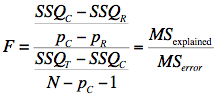
where:
SSQC is the sum of squares for the complete model,
SSQR is the sum of squares for the reduced model,
pC is the number of predictors in the complete model,
pR is the number of predictors in the reduced model,
SSQT is the sum of squares total (the sum of squared deviations of the criterion variable from its mean), and
N is the total number of observations
The degrees of freedom for the numerator is pC - pR and the degrees of freedom for the denominator is N - pc -1. If the F is significant, then it can be concluded that the variables excluded in the reduced set contribute to the prediction of the criterion variable independently of the other variables.
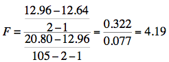
This formula can be used to test the significance of R2 by defining the reduced model as having no predictor variables. In this application, SSQR and pR = 0. The formula is then simplified as follows:
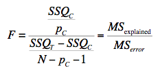
which for this example becomes:
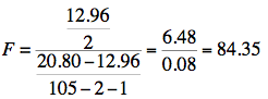
The degrees of freedom are 2 and 102.
The F distribution calculator shows that p
< 0.001.
F Calculator
The reduced model used to test the variance explained uniquely by a single predictor consists of all the variables except the predictor variable in question. For example, the reduced model for a test of the unique contribution of HSGPA contains only the variable SAT. Therefore, the sum of squares for the reduced model is the sum of squares when UGPA is predicted by SAT. This sum of squares is 9.75. The calculations for F are shown below:
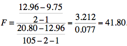
The degrees of freedom are 1 and 102.
The F distribution calculator shows that p
< 0.001.
Similarly, the reduced model in the test for the unique contribution of SAT consists of HSGPA.
The degrees of freedom are 1 and 102.
The F distribution calculator shows that p
= 0.0432.
The significance test of the variance explained uniquely by a variable is identical to a significance test of the regression coefficient for that variable. A regression coefficient and the variance explained uniquely by a variable both reflect the relationship between a variable and the criterion independent of the other variables. If the variance explained uniquely by a variable is not zero, then the regression coefficient cannot be zero. Clearly, a variable with a regression coefficient of zero would explain no variance.
Other inferential statistics associated with multiple regression are beyond the scope of this text. Two of particular importance are (1) confidence intervals on regression slopes and (2) confidence intervals on predictions for specific observations. These inferential statistics can be computed by standard statistical analysis packages such as R, SPSS, STATA, SAS, and JMP.
SPSS Output JMP Output
Assumptions
No assumptions are necessary for computing the regression coefficients or for partitioning the sum of squares. However, there are several assumptions made when interpreting inferential statistics. Moderate violations of Assumptions 1-3 do not pose a serious problem for testing the significance of predictor variables. However, even small violations of these assumptions pose problems for confidence intervals on predictions for specific observations.
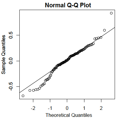
- Residuals are normally distributed:
As in the case of simple linear regression, the residuals are the errors of prediction. Specifically, they are the differences between the actual scores on the criterion and the predicted scores. A Q-Q plot for the residuals for the example data is shown below. This plot reveals that the actual data values at the lower end of the distribution do not increase as much as would be expected for a normal distribution. It also reveals that the highest value in the data is higher than would be expected for the highest value in a sample of this size from a normal distribution. Nonetheless, the distribution does not deviate greatly from normality.
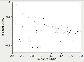
- Homoscedasticity:
It is assumed that the variances of the errors of prediction are the same
for all predicted values. As can be seen below, this assumption is violated in the example data because the errors of prediction are much larger for observations with low-to-medium predicted scores than for observations with high predicted scores. Clearly, a confidence interval on a low predicted UGPA would underestimate the uncertainty.
- Linearity:
It is assumed that the relationship between each predictor variable and the criterion variable is linear. If this assumption is not met, then the predictions may systematically overestimate the actual values for one range of values on a predictor variable and underestimate them for another.
Please answer the questions:
|