If you are having problems with Java security, you might find
this page helpful.
Learning Objectives
- Develop a basic understanding of the properties of a sampling distribution based on the properties of the population.
Instructions
This simulation illustrates the concept of a sampling distribution. Depicted on the top graph is the population from which we are going to sample. There are 33 different values in the population: the integers from 0 to 32 (inclusive). You can think of the population as consisting of having an extremely large number of balls with 0's, an extremely large number with 1's, etc. on them. The height of the distribution shows the relative number of balls of each number. There is an equal number of balls for each number, so the distribution is a rectangle.
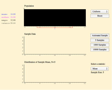
If you push the "animated sampling" button, five balls are selected and and are plotted on the second graph. The mean of this sample of five is then computed and plotted on the third graph. If you push the "animated sampling" button again, another sample of five will be taken, and again plotted on the second graph. The mean will be computed and plotted on the third graph. This third graph is labeled "Distribution of Sample Means, N = 5" because each value plotted is a sample mean based on a sample of five. At this point, you should have two means plotted in this graph.
The mean is depicted graphically on the distributions themselves by a blue vertical bar below the X-axis. A red line starts from this mean value and extends one standard deviation in length in both directions. The values of both the mean and the standard deviation are given to the left of the graph. Notice that the numeric form of a property matches its graphical form.
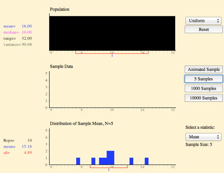
The sampling distribution of a statistic is the relative frequency distribution of that statistic that is approached as the number of samples (not the sample size!) approaches infinity. To approximate a sampling distribution, click the "5,000 samples" button several times. The bottom graph is then a relative frequency distribution of the thousands of means. It is not truly a sampling distribution because it is based on a finite number of samples. Nonetheless, it is a very good approximation.
The simulation has been explained in terms of the sampling distribution of the mean for N = 5. All statistics, not just the mean, have sampling distributions. Moreover, there is a different sampling distribution for each value of N. For the sake of simplicity, this simulation only uses N = 5. Finally, the default is to sample from a distribution for which each value has an equal chance of occurring. Other shapes of the distribution are possible. In this simulation, you can make the population normally distributed as well.
In this simulation, you can specify a sample statistic (the default is mean) and then sample a sufficiently large number of samples until the sampling distribution stabilizes. Make sure you understand the difference between the sample size (which here is 5) and the number of samples included in a distribution.
You should also compare the value of a statistic in the population and the mean of the sampling distribution of that statistic. For some statistics, the mean of the sampling distribution will be very close to the corresponding population parameter; for at least one, there will be a large difference. Also note how the overall shape of sampling distribution differs from that of the population.
Finally, as shown in the video demo, you can change the parent populaton to a normal distribution from a uniform distribution.
Video Instructions
Video Demo
The video below demonstrates the use of the Sampling distribution Demonstration. The first graph represents the distribution of the population from which the sample will be drawn. In the video this distribution is changed to normal. Each time the "Animated Sample" button is clicked a random sample of five elements is drawn from the population. You can draw multiple samples of 5 by clicking on the buttons directly below "Animated Sample". The mean of each of these sample is displayed in the third graph on at the bottom. The graph can also be set to display other descriptive statistics besides the mean.
If you look to the left of this third graph you can see the mean and standard deviation of the sampling distribution. Try drawing 50,000 samples from both types of population distributions and compare the sampling distribution statistics to their equivalent population statistics to see if you can discover any trends.
Video Demo