Group Differences Demonstration
Each applicant for a job is given a series of tests and interviews
from which a numerical "suitability" score is calculated. This score
is designed to predict success on the job and is used as the
criterion for selecting applicants.
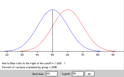
The applicants are from two demographic groups represented by the
blue and red distributions. The same number of people are in each
group. The blue distribution has a mean of 50; the red distribution
has a mean of 60. Both distributions have standard deviations of 10.
Applicants with scores greater than or equal to 50 are hired. The
figure shows that among people hired, there are 1.683 people from the
red distribution for each person from the blue distribution. The
difference between the groups explains 20% of the variance.

The mean of the blue distribution and the standard deviations of the
distributions are fixed. You can change the mean of the red
distribution and the cutoff for hiring. (Not on this page; the graph
here is static. Go back to the previous
page to make the changes.) Explore the effects of these
variables. Pay special attention to the effect of a high cutoff.
Simulate the following situation. Males and females are, on average,
equally suitable for a job. However, there is a small gender bias in
the evaluation procedure so that the mean for males is 0.10 standard
deviations (1 point) higher than that for females. This is generally
considered a very small difference since it explains only 0.20% of
the variance. Consider the effect of this small difference if
applicants have to score two or more standard deviations (20 points)
above the female mean to be hired. The EEOC considers a ratio of 1.25
: 1 to be adverse impact. What does this say about the size of a
difference needed to produce adverse impact when only very highly
qualified applicants are hired? Explore other effect sizes and
cutoffs.
