|
Difference between Means
Author(s)
David M. Lane
Prerequisites
Sampling
Distribution of Difference between Means, Confidence
Intervals, Confidence Interval on the
Mean
Learning Objectives
- State the assumptions for computing a confidence interval on the difference
between means
- Compute a confidence interval on the difference between means
- Format data for computer analysis
It is much more common for a researcher to be
interested in the difference between means than in the specific
values of the means themselves. We take as an example the data
from the "Animal
Research" case study. In this experiment, students rated
(on a 7-point scale) whether they thought animal research is wrong.
The sample sizes, means, and variances are shown separately for
males and females in Table 1.
Table 1. Means and Variances in Animal Research study.
|
Condition
|
n
|
Mean
|
Variance
|
|
Females
|
17
|
5.353
|
2.743
|
|
Males
|
17
|
3.882
|
2.985
|
As you can see, the females rated animal research
as more wrong than did the males. This sample difference between
the female mean of 5.35 and the male mean of 3.88 is 1.47. However,
the gender difference in this particular sample is not very important.
What is important is the difference in the population.
The difference in sample means is used to estimate the difference
in population means. The accuracy of the estimate is revealed
by a confidence
interval.
In order to construct a confidence interval, we
are going to make three assumptions:
- The two populations have the same variance. This assumption
is called the assumption of homogeneity of
variance.
- The populations are normally
distributed.
- Each value is sampled independently
from each other value.
The consequences of violating these assumptions are discussed in
a later section. For now, suffice it to say that small-to-moderate
violations of assumptions 1 and 2 do not make much difference.
A confidence interval on the difference between
means is computed using the following formula:
Lower Limit = M1 -
M2 -(tCL)( ) )
Upper Limit = M1 - M2
+(tCL)()
where M1 - M2
is the difference between sample means, tCL
is the t for the desired level of confidence, and
is the estimated standard
error of the difference between sample means. The meanings
of these terms will be made clearer as the calculations are demonstrated.
We continue to use the data from the "Animal
Research" case study and will compute a confidence interval
on the difference between the mean score of the females and the
mean score of the males. For this calculation, we will assume
that the variances in each of the two populations are equal.
The first step is to compute the estimate of the
standard error of the difference between means ().
Recall from the relevant
section in the chapter on sampling distributions that the
formula for the standard error of the difference in means in the
population is:

In order to estimate this quantity, we estimate
σ2 and use that estimate in place
of σ2. Since we are assuming the
population variances are the same, we estimate this variance by
averaging our two sample variances. Thus, our estimate of variance
is computed using the following formula:

where MSE is our estimate of σ2.
In this example,
MSE = (2.743 + 2.985)/2 = 2.864.
Note that MSE stands for "mean square error" and is the mean squared deviation of each score from its group's mean.
Since n (the number of scores in
each condition) is 17,
= = = = 0.5805.
The next step is to find the t to use for the
confidence interval (tCL). To calculate
tCL, we need to know the degrees
of freedom. The degrees of freedom is the number of
independent estimates of variance on which MSE is based. This
is equal to (n1 - 1) + (n2
- 1) where n1 is the sample size of the
first group and n2 is the sample size
of the second group. For this example, n1=
n2 = 17. When n1=
n2, it is conventional to use "n"
to refer to the sample size of each group. Therefore, the degrees
of freedom is 16 + 16 = 32.
Online:
Calculator: Find t for confidence interval
From either the above calculator or a t table, you can find that
the t for a 95% confidence interval for 32 df is 2.037.
We now have all the components needed to compute
the confidence interval. First, we know the difference between
means:
M1 - M2
= 5.353 - 3.882 = 1.471
We know the standard error of the difference between
means is
= 0.5805
and that the t for the 95% confidence interval
with 32 df is
tCL = 2.037
Therefore, the 95% confidence interval is
Lower Limit = 1.471 - (2.037)(0.5805) = 0.29
Upper Limit = 1.471 + (2.037)(0.5805) = 2.65
We can write the confidence interval as:
0.29 ≤ μf - μm
≤ 2.65
where μf is the population mean for
females and μm is the population mean
for males. This analysis provides evidence that the mean for females
is higher than the mean for males, and that the difference between
means in the population is likely to be between 0.29 and 2.65.
Formatting data for Computer Analysis
Most computer programs that compute t tests require
your data to be in a specific form. Consider the data in Table 2.
Table 2. Example Data.
|
Group 1
|
Group 2
|
|
3
|
5
|
|
4
|
6
|
|
5
|
7
|
Here there are two groups, each with three observations. To format
these data for a computer program, you normally have to use two
variables: the first specifies the group the subject is in and the
second is the score itself. For the data in Table 2, the reformatted
data look as follows:
Table 3. Reformatted Data.
|
G
|
Y
|
|
1
|
3
|
|
1
|
4
|
|
1
|
5
|
|
2
|
5
|
|
2
|
6
|
|
2
|
7
|
To use Analysis
Lab to do the calculations, you would copy the data and then
- Click the "Enter/Edit User Data" button. (You may
be warned that for security reasons you must use the keyboard
shortcut for pasting data.)
- Paste your data.
- Click "Accept Data."
- Set the Dependent Variable to Y.
- Set the Grouping Variable to G.
- Click the t-test confidence interval button.
The 95% confidence interval on the difference between means extends
from -4.267 to 0.267.
Computations for Unequal Sample Sizes (optional)
The calculations are somewhat more
complicated when the sample sizes are not equal. One consideration
is that MSE, the estimate of variance, counts the sample with
the larger sample size more than the sample with the smaller sample
size. Computationally this is done by computing the sum of squares
error (SSE) as follows:

where M1 is the mean for group 1 and
M2 is the mean for group 2. Consider
the following small example:
Table 4. Example Data.
|
Group 1
|
Group 2
|
|
3
|
2
|
|
4
|
4
|
|
5
|
|
M1 = 4 and M2 = 3.
SSE = (3-4)2 + (4-4)2 + (5-4)2 + (2-3)2 + (4-3)2 = 4
Then, MSE is computed by: MSE = SSE/df
where the degrees of freedom (df) is computed as before:
df = (n1 -1) + (n2 -1) = (3-1) + (2-1) = 3.
MSE = SSE/df = 4/3 = 1.333.
The formula
=
is replaced by
=
where nh is the harmonic mean of the sample sizes and is computed
as follows:
nh = 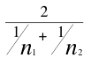 = =
 = 2.4
= 2.4
and
=
 = 1.054.
tCL for 3 df and the 0.05 level = 3.182.
Therefore the 95% confidence
interval is
Lower Limit = 1 - (3.182)(1.054)= -2.35
Upper Limit = 1 + (3.182)(1.054)= 4.35
We can write the confidence interval
as:
-2.35 ≤ μ1 - μ2
≤ 4.35
Please answer the questions:
|