Instructions for SAS JMP
Inputing the data
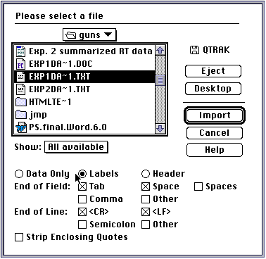
Start JMP and go to the file Menu Choose "Import" and then choose "Text/Other..." When the window opens, Select the labels option (this is done because the text based dataset includes the column titles) and the Dataset for this study (you may have to save it to a local drive).

JMP should open a Data editor window that has the correct column titles:
If the names aren't right, just hilight the names by double clicking on the bold face column titles and then type in the appropriate names.
The dataset that was imported has each group in separate columns. Before you can run the Quantile plots the data must be re- arranged. Simply choose "Tables" and then choose the "Stack Columns" option. Choose the columns aw, an, cxew, and cxen. JMP will have default titles for the two new columns which you may change now or when the coluns actually appear in the chart.
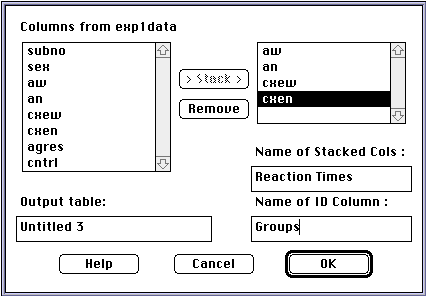
JMP will then open a new data editor window with the new columns:

Now, to get the plots, First, in the menu choose "Analyze" and then "Fit Y by X" then you will find the following window:
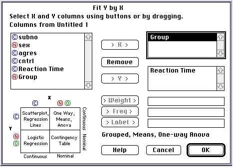
Make sure that you choose the continuous variable as the Y variable and the group variable as the X variable - here the continuous variable is Reaction Times" and the group variable is called "Group"
when you first click OK the output window looks like this:
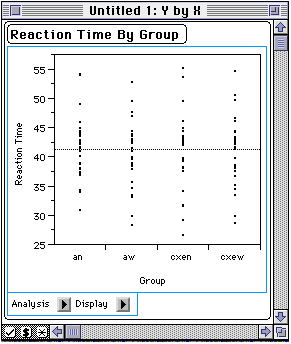
To get the quantile plots, click the ![]() arrow. A list
of options will then appear. You will notice that the "Show points" opotion
is selected. Deselect the "Show Ponts" option, and then use the mouse so
the "Quantile Boxes" and "Mean Dots, Error Bars" options are
checked.
arrow. A list
of options will then appear. You will notice that the "Show points" opotion
is selected. Deselect the "Show Ponts" option, and then use the mouse so
the "Quantile Boxes" and "Mean Dots, Error Bars" options are
checked.
Proceed the same as you did for the quantile plots.
When you get the output window, choose the ![]() button and make
sure the "Means, Std dev, Std err" option is selected.
button and make
sure the "Means, Std dev, Std err" option is selected.
To get more detailed statistics, we need to have the data in it's original form.
(If you did not save the original, you can either re-open the original data set or
you can unstack the column using the "Tables" and then the "Split
Columns" option.) When you are dealing with the original data table, click
the right square at the top of the column "aw" and select "Y".
Do this for " an", "cxew", and "cxen"
as well. Then go to "Analyze" on the menu bar and choose the
"Distribution of Y" option. When the output window opens select
the ![]() beside the "Moments" button and select the
"More Moments" option.
beside the "Moments" button and select the
"More Moments" option.
To get the Normal Probability Plots for "aw", " an", "cxew", and "cxen", go to the top of each column and click and hold the mouse button on the right square. Select "Y". Then go to the menu bar and click on the "Analyze" option. Then drag the cursor to "Distribution of Y". Look at the bottom left corner of the output window and find the checkmark (See below)

Click on the checkmark and select "Normal Quantile Plot". To see just the Normal Quantile Plot, simply de-select all the other options under the checkmark.
For this procedure, the original format of the data - one column for each group. Select the four columns aw, an, cxew, and cxen as "Y" variables and choose the "Fit Model" option from the "Analyze" menu This should give the following window:
![]()
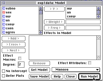
Note: if you did not choose the 4 variables as "Y" in the data spreadsheet - you can do that in this window. Simply click the variable name from the left subwindow and drag it into the top right window for the "Y" variables. Make sure that the Manova selection is made. Clicking the "Run Model" button will give you the following window:
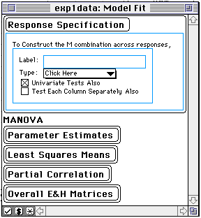
To do the 2-way within subjects analysis - click on ![]() to
get a list of options. Choose the Compound option and you will get the following
window.
to
get a list of options. Choose the Compound option and you will get the following
window.
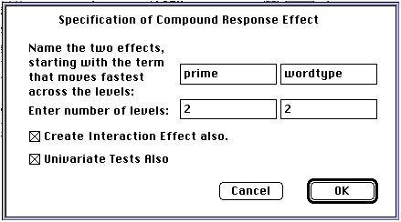
Then go back to the original window expdata1: Model Fit (expdata1 is the name of the data spreadsheet used for the analysis) and enlarge it and you will find the output.
The dependent variable needed for this analysis is the difference between two
priming scores:
1. Aggresive word neutral prime - Aggressive word weapon prime
2. Non-aggresive word neutral prime - Non-aggressive word weapon prime
To compute this dependent variable, do the following:
Using the data editor with the initial input, click the "Cols"
menu and then choose the "New Columns"option. Then go to Data source
and select the "Formula" option. Change the "Col name"
to a name that represents the variable that you want. Here it is called "difference."
When you are done the window should look like this:
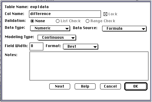
Now click "OK". The next window to pop up will be the formula window: To create the differences of differences as described previously , click the left parenthesis button and then the first variable name "an" and then click the minus sign button... Continue in this manner until you get the formula (an - aw) - (cxen - cxew). Then click the "Evaluate" button and close the window. When you look at the original data table you will now see the new column appended to the end:

To have JMP perform the t-test, go to the menu bar and select "Analyze" andthen select "Distribution of Y's"
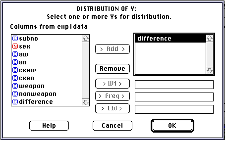
Choose "difference" from the names of the columns by clicking and dragging it from the "Columns from..." subwindow to the window on the right. Then click "OK" The following analysis window should open up:
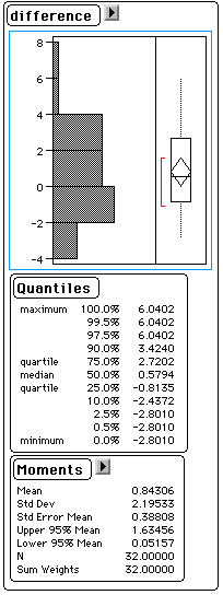
click the ![]() beside the "difference"
button. Select the "Test Mean=value" option and then the next window
to pop up should ask for a value that you want to test. with default value being
0.0. Since you are testing if the difference is different from zero, just
click "OK" and then the t-test is reported.
beside the "difference"
button. Select the "Test Mean=value" option and then the next window
to pop up should ask for a value that you want to test. with default value being
0.0. Since you are testing if the difference is different from zero, just
click "OK" and then the t-test is reported.
If we want to investigate the effect gender has on the results, we must include a between subjects portion of the design with the within subjects design. This can be done with a Between-Within Subjects Anova. Having JMP perform a between-within ANOVA is very similar to the within ANOVA. The only difference is that you select the between variable(s) as "X" variables in the top of the column. Then just as with the Within subject 2-way anova you choose the "Fit Model" option under the "Analyze" menu.
This time your window should look like this:
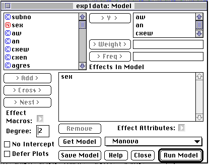
Notice that now the variable "sex" appears in the "Effects In Model" section. If it does not, simply use the mouse to click on the variable "sex" and then drag it into the appropriate box. Then, from this window you proceed the same as you did for the Within 2-way ANOVA.