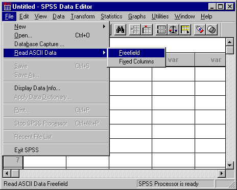
The first thing you have to do is to copy the data into a file. You can do this by going to the menu bar in your browser and select "Edit" then "Select all" after you have opened the data in your browser. Next paste it into some text editor or word processor that can save as a text only file. Next open SPSS, and on the"Data Editor" window, go to the "File" option on the menu bar and select "Read ASCII Data" from the pull down menu and "Freefield" from the pop up menu (as shown below).
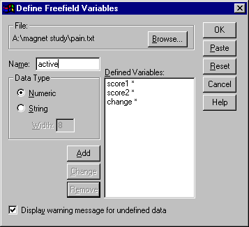
This will open the "Define Freefield Variables" dialog box. Click on the "Browse" button in the "File" box and find the file name you saved the data to. Then click on the "Name" slot. Type "score1", make sure that "Numeric" is selected under "Data Type", then click the "Add" button to name the first column of your data editor score1. Repeat this process, typing "score2", "change", and "active". Even though "active" is a categorical variable, the original researcher recorded active using the values 1 and 2, so we want SPSS to read it as a number. After you have added "active" to the "Defined Variables:" list, click "OK".
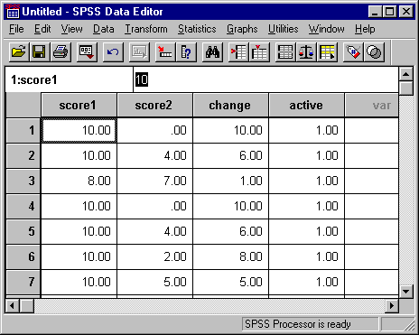
Now your data should appear in the "Data Editor" but notice that the top line is blank, except for a period (.) in each cell. Remove this by clicking on the "1" square in the left most column. This should highlight the entire first row (shown below). While the row is selected, press the "Delete" key to delete the empty row.
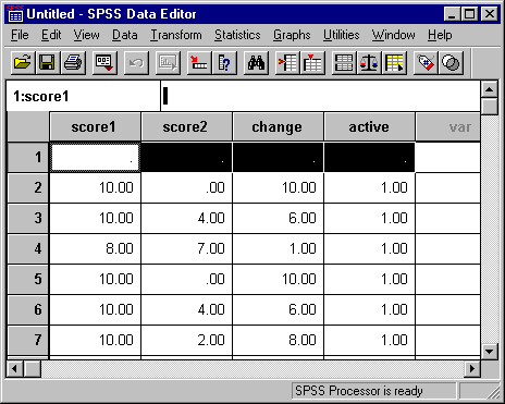
When you are finished the "Data Editor" should appear as shown below.
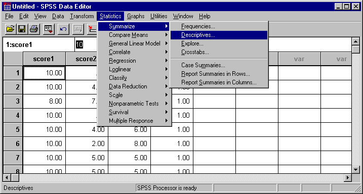
Go to the "Statistics" option on the menu bar of the data editor window. Then go to "Summarize" on the pull down menu, and then choose "Descriptives..." as shown below.
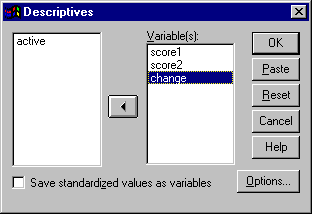
This will open the "Descriptives" dialog box (shown below). On the left will be a box containing all of the variables in the data worksheet and on the right will be a box titled "Variable(s)". Move the variables for which you desire the descriptive statistics to the "Variable(s)" box by first selecting the variable and then clicking the arrow button in between the two variables. The picture below shows how the dialog box should look to calculate the Descriptives for "score1", "score2" and "change". Then click "Options..."
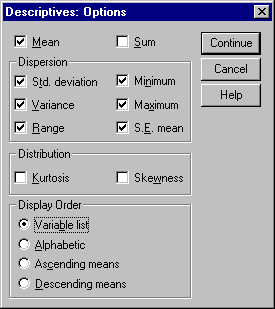
This opens the "Descriptives: Options" dialog box (shown below). In this dialog box, you determine the actual descriptive statistics to be calculated. Simply check the desired descriptives and then click "Continue". This brings you back to the "Descriptives" dialog box, and here simply click "OK".
Detailed Descriptive Statistics
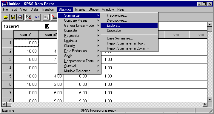
Go to the "Statistics" pulldown menu in the SPSS window. Then go to the "Summarize" menu, and finally choose "Explore..." (Shown Below)
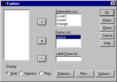
After selecting "Explore" a dialog box should open containing a list of the variables on the left, and three blank boxes on the right with the titles "Dependent List:", "Factor List:", and "Label Cases by:" on top. Move the variables that you want the descriptives calculated for into the "Dependent List:" box by first clicking the variable, and then clicking the arrow button beside the desired box. In a similar manner, put the grouping variable in "Factor List:". Below is a picture of how the dialog box would look if one were to compute the descriptives on "score1", "score2", and "change", grouped by "active".
Next we want to choose what statistics we want calculated. Click on "Statistics...". This will open another dialog box (shown below)
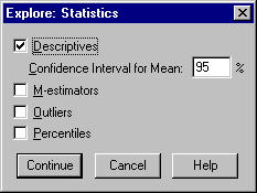
Make sure the "Descriptives" box is checked, and then click "Continue". This brings you back to the "Explore" dialog box. We also want to look at the box plots and normal probability plots, so we can do that by clicking the "Plots" button. Doing so gives us the following dialog box:
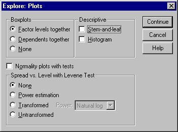
Since three variables we are exploring are grouped by "active", it makes sense to put the box plots side by side for each level of "active". to do this, select "Factor levels together" in the "Box plots" section of the dialog box. To get normal probability plots, check the box beside "Normal Probability Plots with tests". "Stem-and-leaf will be checked in the "Descriptives" section by default. You can click on it to remove the check. Since we are performing a box plot and a normal probability plot, a stem-and-leaf plot would be redundant.
Box plots and Normal probability plots can also be done separately, and the procedure for doing so is described below.
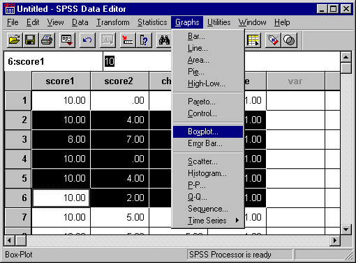
To create a box plot in SPSS, simply go to the "Graphs" option, then select "Box plot" from the pull-down menu (shown below).
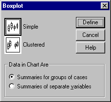
Doing this will open up the "Boxplot" dialog box, (shown below). For the magnet experiment, we are comparing "score2", and "change" grouped by "active". Therefore we select "Simple" and make sure that "summaries for groups of cases" is selected. Then click the "Define" button.
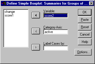
This will open up another dialog box with the list of variables on the left and three slots in a column on the right. In the slot titled "Variable" put the variable you want to be plotted by selecting it in the column on the left and clicking the arrow beside the "Variable" slot. (For this experiment, you will want to do this with either "score2" and "change".) Next select the grouping variable (in this experiment, "active"), and click the arrow next to the slot labeled "Category Axis." Then click the "OK" button. Below is a picture of what the dialog box should look like for the boxplots for "score2" grouped by "active".
We want to create normal probability plots for "score2" and "change" grouped by "active".
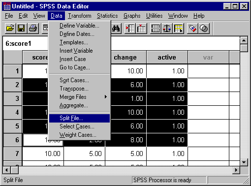
To do this, first go to the "Data" option on the menu, then
choose "Split file" from the pull down menu. (Shown Below)
This opens the "Split File" dialog box. With the mouse select "Compare groups" and then move the grouping variable from the list a the left of the dialog box into the box labeled "Groups Based on:". To do this, click on the grouping variable in the left box and then click the arrow beside the "Groups Based on:" box (shown below). Make sure also that "Sort the file by grouping variables" is also selected. Click "OK" This just told SPSS that you will be looking at all your variables broken into groups by the grouping variable. In this specific example, the variables are grouped by "active".
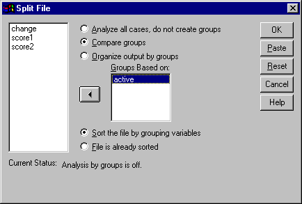
note: the "current status" won't change until you click "OK".
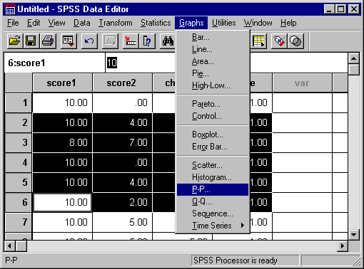
Now we are ready to create P-P plots using SPSS. Go to the "Graphs" option on the menu bar on the data editor. Then choose "P-P..." from the pull down menu (shown below)
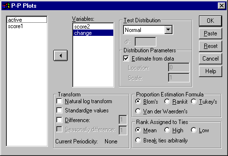
This opens the "P-P Plots" dialog box. From the column on the left, choose the variables you want to graph. Select one variable that you want to plot then click the arrow beside the box labeled "Variables". Repeat this until all desired variables are in the "Variables" box. Also make sure that "Normal" appears in the "Test Distribution" slot. Then click "OK". The dialog box shown below will generate P-P Plots for "score2" and "change", and if you also followed the above instructions, you will get 4 plots, 1 for "score2", "active" = 1; one for "score2" "active" = 2; one for "change", "active"=1; and one for "change", "active" = 2.
Note:. Note: SPSS also gives a detrended normal probability plot. This is basically a plot of the residuals from the reference line. The way to interpret it is the same as any other residual plots. The further away from zero the residuals are, the less normal the sample is. But this is beyond the level of this demonstration, and has been omitted from this web page
Note: Before continuing our analysis in SPSS, You may want to turn off the global grouping that we did for the P-P plots. to do this go back to the "Data" option on the menu bar of the data editor window. Choose "Split File..." from the pull down menu to get back to the "Split File" dialog box:
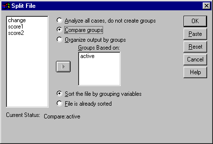
Select "Analyze all cases, do not create groups" and then click "OK" to undo the global grouping. In some of the later analysis, the statistic function itself will ok at groups via a grouping variable declared at that time.
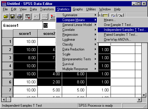
To perform a T-test, simply choose "Statistics" from the menu bar of the data editor, then choose "Compare Means" from the pull down menu, and then choose "Independent-Samples T Test..." from the next level of pull down menus. (Shown below)
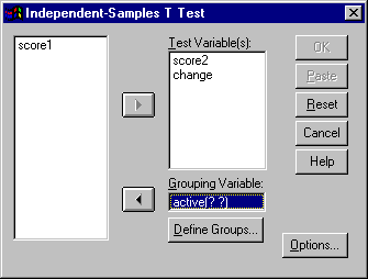
This should give you the "Independent-Samples T Test" Dialog box, with the familiar boxes of variables. On the left are the available variables, and on the right, put the variables you want to test. Select the variable you want to test and then click the right arrow beside the box labeled "Test Variable(s)". Then select the grouping variable from the column on the left and click the arrow beside the slot labeled "Grouping Variable". The dialog box should appear as below:
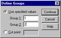
Click "Define Groups..." This opens the "Define Groups" Dialog box pictured below. Recall the paradigm of the magnet study had "active" = 1 refer to those subjects who had an active magnetic device, and "active" = 2 refer to those subjects with a placebo device. Use these values in the "Group 1" and "Group 2" slots. Then click "Continue".
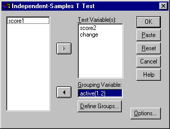
Now you should be back to the "Independent-Samples T Test" dialog box. Click "OK" to perform the T test.
ANOVA (General Linear Model) Repeated measure
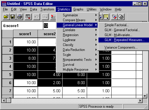
To perform an ANOVA, select the "Statistics" option on the menu. Next select "General Linear Model" on the pull down menu, and finally select "GLM-Repeated Measures..." on the next level of pull down menu. (Shown below.)
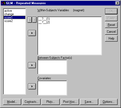
This opens the "GLM-Repeated Measures Define Factor(s)" dialog box. Shown below. Notice how most the buttons are gray indicating that you cannot click any of them yet. The reason for this is that you need to define the factors for your ANOVA paradigm. You can change the name or leave it as factor 1, but the important part is to determine the number of levels of the factor.
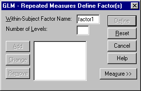
Since we are dealing with "score1" and "score2" as a pre and post treatment measure on the same subject, we have two levels. Fill in "Number of Levels" by clicking the white slot and typing "2".
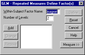
Notice how the "Add" button has darkened. Click the "Add" button.
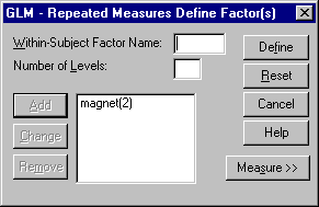
At this point we can create another factor for a more complicated design by repeating the above procedure, but for the magnet example, we are only dealing with a one factor design. When we have named and added all the factors to the middle box (where "magnet(2)" appears in the above picture), click "Define". This opened up the "GLM-Repeated Measures" dialog box, shown below:
For the magnet study we do not really have any between subjects factors so that box should remain empty in the dialog box. Notice that there are two blanks in the "Within-Subjects Variables" box. We need to fill those. Select "score1" in the column on the left and move it into the "Within-Subjects Variables" box by clicking on the arrow beside the "Within-Subjects Variables" box. Then repeat the procedure for "score2". Your dialog box should appear as below when you are all finished:
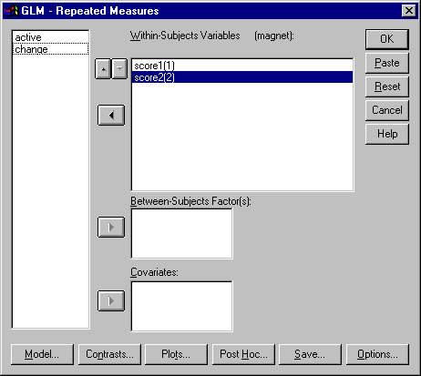
Notice the number in parentheses following the variables of "score1" and "score2". It would be a good idea whenever dealing with pre-treatment and post treatment scores to move the pre treatment variable into the "Within-Subjects Variables" box first and then move in the post-treatment score. That way the 1 and 2 will correspond with pre and post treatment scores appropriately. Now Click "OK" to perform the procedure.
We need to input a new set of data for performing a chi square on the magnet data (for an explanation of the paradigm, go to the page about inferential statistics). Here is a simple way to put in categorical data. First open a new data window by going to the "File" option on the data editor window and select "New" from the pull down menu. Next input the data with one column labeled "improve", one column labeled "active", and one column labeled "counts" (shown below)

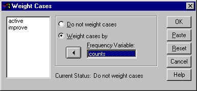
"Improve" and "active" are the categorical variables, and therefore we have 4 groups. I used 1 to refer to "yes", and 2 to refer to "no". "Counts" refers to how many are in each group, and we need to let SPSS know this. Type in the numbers as you see them in the above picture. Go to the "Data" option in the menu at the top of the "Data Editor" window. Then choose "Weight Cases..." from the pulldown menu.

This will open the "Weight Cases" Dialog box. To weight the cases, select "Weight cases by", and then click on the variable that recorded the frequency of the groups, (in this example the frequency variable is "counts") and move it into the "Frequency Variable" slot by clicking the arrow beside the slot. Next click "OK". You can turn off the weight cases option by simply going back to the "Weight Cases" dialog box and choose "Do not weight cases", and click "OK" but we do not want to do that now. The dialog box pictured below shows how to set up the "Weight Cases" using counts as the variables containing weights.
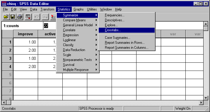
After setting up the weighted cases, then go to the "Statistics" option on the menu bar at the top of an SPSS window. Then choose "Summarize" on the pull down menu and then choose "Crosstabs..." on the pop up menu.
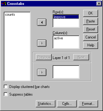
This will open the "Crosstabs" dialog box (shown below). All of your variables should be in a column on the left side of the window. Choose which variable you want to be the category for the columns and which variable you want to be the category for the rows. Then Click the button that says "Statistics...".
This opens the "Crosstabs: Statistics" dialog box. (Shown below) There are many statistics listed here. We are interested in calculating the Chi-square, so make sure that box is checked. For this example, that is the only statistic we want so that is the only box checked. Then click "Continue". This brings you back to the "Crosstabs" dialog box. Click "OK" in this box.

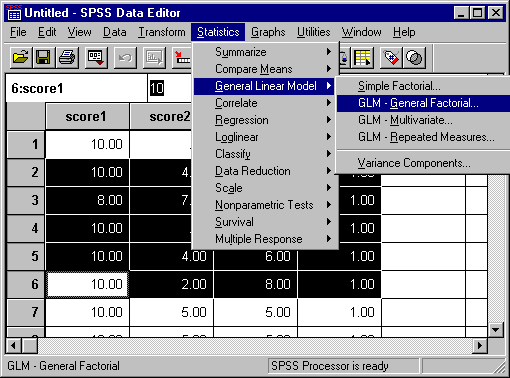
To perform ANCOVA in SPSS go to the "Statistics" option on the menu bar for the "Data Editor" window then choose "General Linear Model" from the pull down menu and choose "GLM - General Factorial..." from the pop - up menu (shown below).
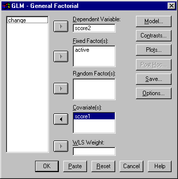
This will open the "GLM-General Factorial" dialog box. All the variables will be in the column on the left side of the dialog box. We need to assign the variables in the appropriate positions for our model. We want "score2" to be our dependent variable so select "score2" on the left by clicking on it, and then click the arrow beside the slot labeled "Dependent Variable". "Active" is our grouping variable, so we want that to be a fixed factor. Select "active" in the left hand column by clicking on it and then click on the arrow button beside the "Fixed Factor(s)" box. Finally we want "score1" to be our covariate for this ANCOVA design, so select "score1" from the left hand column by clicking on it, and move it to the "Covariate(s)" box by clicking on the arrow button beside the box. Then click "Model"
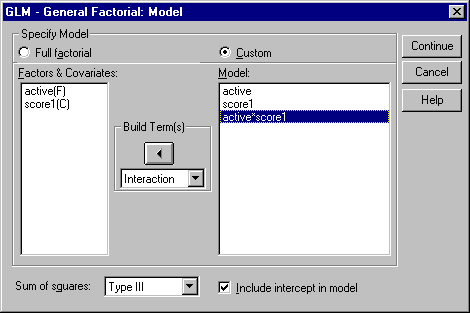
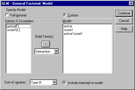
This opens the "GLM - General Factorial: Model" dialog box. Click on "Custom" so a little black dot appears in the circle beside "Custom". Make sure in the "Build term(s)" box "Interactions" is showing. Then select the variables from the "Factors & Covariates" list and move them to the "Model" box the same way you moved the variables in the "General Factorial" box described above. Note that factors are followed by "(F)" and covariates are followed by "(C)". So click on "active", then click the arrow button in the "Build Term(s)" box. Do the same for "score1". To get the interaction term in your model, click both variables you want in the interaction, in this case both "active" and "score1", so that they are simultaneously highlighted. (Shown below).
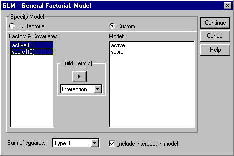
While both are highlighted, click the arrow button in the "Build Term(s)" box. When you are finished, the model box should look like the following picture:
Click "Continue". This brings you back to the "GLM - General Factorial" dialog box. Click "OK" to run the model. With the interaction.
As mentioned above, go to "Statistics" then to "General Linear Model", then to "GLM- General Factorial..." (shown below)
Again this opens the "GLM - General Factorial" dialog box. This box you can leave the same as before (shown below), so just click "Model".
As before, clicking "Model" opens the "GLM - General Factorial: Model" dialog box. This time we want to remove the interaction term from the model. Simply click on the "active*score1" term in the "Model:" column on the right and then click the arrow in the "Build Term(s)" box. This should make that term disappear. Then click "Continue" which brings you back to the "GLM - General Factorial: Model" dialogue box, Click "OK" to run the new model.